
In this tutorial, we are going to cover how to use the INDIRECT Function with named ranges in Excel. Before we begin, please make sure you have a firm understanding on how to use the INDIRECT Function.
For this example, we will be using the following formula.
=INDIRECT(ref_text, [A1])
Before we can proceed, we first need to Name the Range. Please review before continuing.
Once we have named the range/ranges in our table/list, we can proceed with using the INDIRECT function.
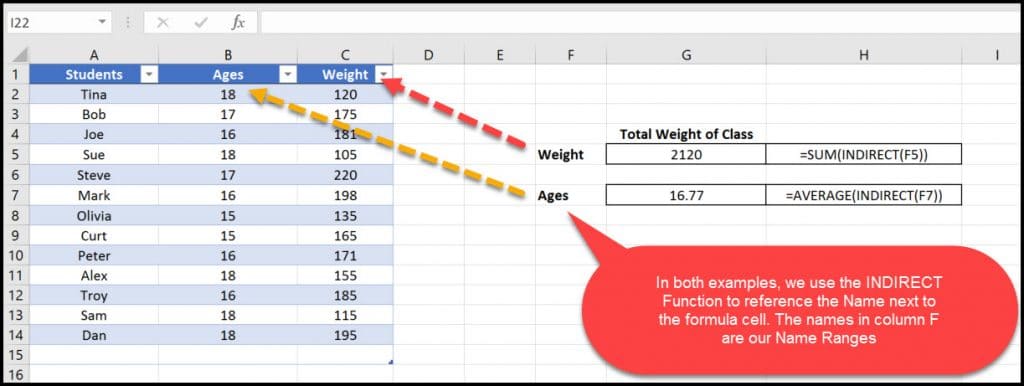
Let’s review the example below. All three columns on our table have been Named. In our scenario, the column Names match the Header Name. Please note that this is not always the case. The names can be adjusted using the Name Manager.
Next, we use the following formulas in cells G5 and G7. Using the Indirect function, we are telling Excel to look at the Name in cell F5 and F7. Excel then matches that name with the name we gave to each column. If matched, Excel will return a desired result. In our example, we are showing how to SUM and AVERAGE the columns.
=SUM(INDIRECT(F5))
=AVERAGE(INDIRECT(F7))
How to INDIRECT with multiple range or selection that are not contagious?
Can post an example of what your referring too?