Overview
Introduction for Named Ranges in Excel
This simple tutorial will show you how to use Named Ranges in Excel. Naming ranges in Excel can be an easy way to keep spreadsheets organized
Names in Excel can refer to multiple cells on a worksheet, a specific value, or an individual formula.
The below sections are broken out to help you understand and master naming cells in Excel. You can follow along by downloading the demonstration file.
How to Name Cells in Excel
The video above shows the steps below.
In the above example, we named the column “Salesdata.” Please note that names are not Case Sensitive. “Salesdata” is the same as “SALESDATA.”
- Highlight the Cell or Cells you want to be named.
- Once highlighted, Click inside the “Name box” above A1.
- Type in a name i.e. Salesdata (Review the naming rules below)
- Press Enter
Rules when Naming Cells
Allowed Characters and Requirements
- First Character Rules: Must be one of the following.
- Letter
- Underscore _
- Backslash \
- Other Character Allowed Rules:
- Letters
- Numbers
- Periods
- Underscore
- Backslash \
- Question Mark ?
Not Allowed Characters:
- Spaces cannot be used.
- Special Characters: !,@,#,$ etc.
- Cell References: $A$3, A134
Name Manager
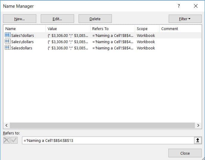
The video above shows the steps below for launching the Name Manager. Depending on a the spreadsheet, you can have dozens of Names being used. The Name Manager allows you to see all of them and make changes as necessary.
- On the Ribbon, Click the Formulas tab, Select Name Manager
- This will bring up the Name Window as shown in Fig 1.1
- From here you can create a New Name, Edit, Delete, or Filter.
Using Named Ranges
Let’s cover how you can use named ranges in Excel. Look at the following example.
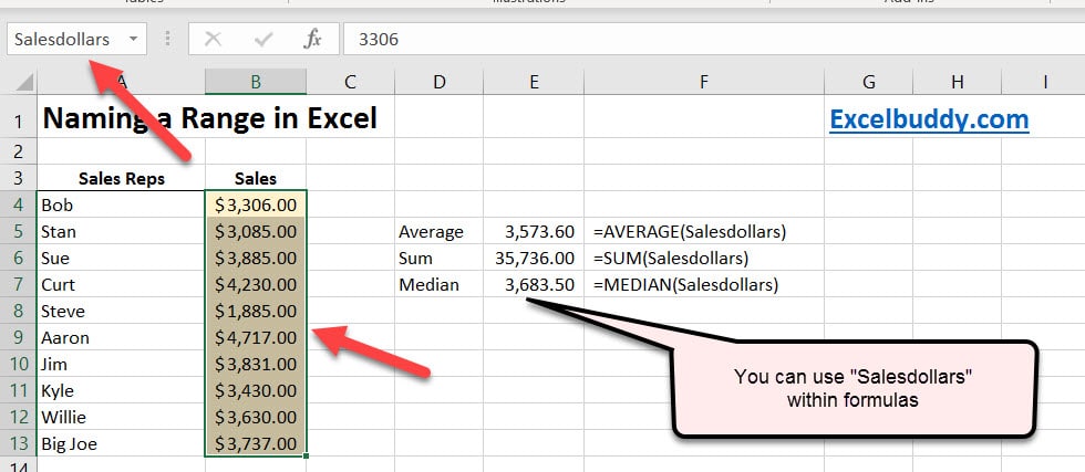
First, highlight the desired range. In our example, this is B4-B13. Next, we name this range “Salesdollars.”
The example below, we show how you use the Named Range with the Average, Sum, and Median function.